Key Concepts Study Tool: Chapter 09

1. Sampling Distribution of Means

Found by repeatedly re-sampling the population and calculating the average values from each sample.
Distribution of means will be tightly clustered around the true population mean.

2. Central Limit Theorem

Any sample statistic (such as the mean) generated from a known population will lie along a normal distribution.
Any one random sample mean should be close enough to the population mean.

central limit theorem

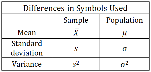
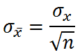
3. Standard Error of the Mean (σ_x̅)

standard error

Think of the standard error as a type of standard deviation, except that instead of measuring how far an observation is from a mean, it refers to the distance that a sample mean is from a population mean.

4. Confidence Intervals

Confidence intervals give a range for the mean and the probability that the true score is within that range.
Confidence limits give the upper and lower ranges of the “confidence interval.”
If population standard deviation is known: Confidence Interval = (x̅) ± (z_critical* X_x̅)
If population standard deviation is unknown: Confidence Interval = (x̅) ± (z_critical* s_x̅)
Where, z_critical,/em> is found in the z-table (Appendix A), σ_x̅ is the population standard error, and s_x̅is the sample standard error. ±

5. The t-Distribution

An infinite number of curves, one for every sample size greater than or equal to two. As sample size increases, the t-distribution increasingly resembles the standard normal distribution.
Values for the t-distribution can be derived by using one of the following equations (when the mean = 0 and the variance is > 1).

t-distribution

6. Degrees of Freedom

All but one of the values are uncertain, or free, because the final value is always known by subtracting the cumulative total of contributions from the total.
When working with the mean: df = n – 1
At df = 120 the values of t- and z-distribution are identical; t should only be used when the n < 120.

7. Estimating a Population Mean with a Known Confidence Interval

Calculate the sample mean.
Assuming that the population standard deviation (σ_x) is known, calculate the standard error of the sample mean using the following equation:
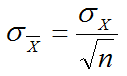
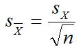
Or, you’ll need to rely on the sample standard deviation and use this equation:
Find the relevant value of z_critical in the z-table in Appendix A that corresponds with a 95 percent confidence interval (1.96 for 95 per cent, 2.58 for 99 per cent in a two-tailed test).
Insert the relevant values into one of the following equations:

8. Estimating Population Proportions Using Only Sample Characteristics

Estimate the standard error of the sample mean:
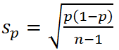
Use df = n – 1 to calculate the degrees of freedom to find the critical value of z, or t, to find the desired confidence interval: CI = P ± z_critical * S_p
It will be necessary to do this for both upper and lower bounds (which explains why ± appears in the equation), meaning that you will have to solve the equation for a positive and negative value of z_critical