
Key Concepts Study Tool: Chapter 16
Click on each concept below to check your understanding.
1. Ordinary Least Squares Regression
- The Formula of Regression:

- The regression line attempts to minimize errors (e = Yi – Ŷi) by creating a line of best fit where the average distance between observations above the line are the same as, or as close as possible to, those below the line.
- Regression allows you to predict the value of the dependent variable (DV) by using the information provided in independent variables (IVs).
- Positive errors: those above the line, due to underestimation
- Negative errors: those below the line, due to overestimation
2. Regression: The Formula
- The equation for the line of best fit is:
- Coefficient: a number or quantity that expresses the nature of the relationship between an independent variable and the dependent variable.
- y-intercept: the value where the regression line crosses the y-axis a = ȳ – bx̄
- error e: defined as e = Y – ŷ, where ŷ is the predicted value.
- Partial slope coefficients (b): the slope assigned to any given independent variable holding all the other independent variables constant.
3. How to Calculate Regression with One Independent Variable
- Find the mean for each X and Y variable.
- Subtract the mean from the value for each observation.
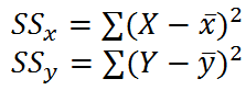
- Square and sum these terms. Each value is known as the sum of squares:
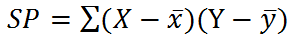
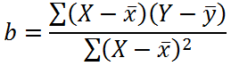
- Find the sum of products:
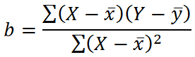
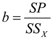
- Calculate b (the partial slope):
- Calculate a (the y-intercept):
- Calculate r:
4. Multiple Regression
- Typically, models will have more than one independent variable. The same equations are used for these models, however with more considerations.
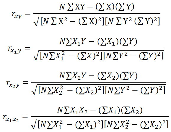
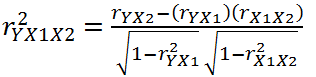
- Once zero-order correlations have been calculated, equations for the partial correlation coefficient are needed.
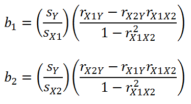
- s = the standard deviation of certain variables
- r = the correlations between them.
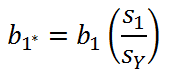
5. Standardized Partial Slopes (beta-weights or b*)
- To compare the relative effects of independent variables that are not measured in the same units, a beta weight (b*) needs to be computed.
- Beta weights show how much change there is to standardized scores of Y when there is a one-unit change in the standardized scores of each independent variable (X), controlling for the effects of all other independent variables.
- To calculate beta-weights:
6. The Multiple Correlation Coefficient
- The multiple correlation coefficient shows the cumulative effect of several independent variables on one dependent variable.
- The correlation of independent variables must be accounted for in the calculation of Pearson’s r-squared (R2). The equation:
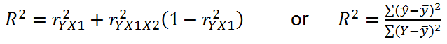
- To calculate R2, we need to calculate:
7. Requirements/Assumptions of Ordinary Least Squares Regression (OLS)
- The DV is interval/ratio, and all independent variables are interval/ratio, dichotomous, or dummy.
- All error terms are normally distributed.
- There is linearity between variables.
- There is homoscedasticity.
8. Creating and Working with Dummy Variables
- Nominal and ordinal level variables must be treated differently in regression.
- If these variables have two response categories (referred to as dichotomous, binary, or dummy variables), the “distance” between categories can be measured.
- Variables with multiple categories can be broken down into a series of dichotomous variables to be entered into a regression equation.
- Only k-1 dummy variables should be included in the equation, (where k = number of response categories in original variable). The reference group refers to the group excluded from the equation, to which coefficients are compared to or referenced to.
9. Identifying the Statistical Significance of One Regression Slope Coefficient
- Calculate the regression slope coefficient:
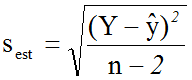
- Determine the squared estimate error:
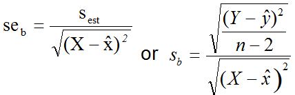
- Calculate the standard error for b using either of the following equations:
- Generate tobserved as and compare tobserved to tcritical, found in Appendix B at df = n – 2