Key Concepts Study Tool: Chapter 18

1. Influential Cases as a Source of Error

Any case that exerts an extraordinary amount of influence on the slope and intercept.
There are two types of influential cases:

Outlier: the distance an observation is from its estimated Y-value (the distance between Y_i and ŷ is huge)
Leverage: measures the distance between an X-value and the mean for that variable (the gap between X_i and x̄)

2. Cook’s Distance (Cook’s D)

Introduced in the late 1970s by Dennis Cook.
Determines the extent to which coefficient estimates (both slopes and intercepts) will change if a particular observation is removed from the analysis.
Values are meaningless by themselves, but any value below 1 is regarded as being tolerable for influence.
Any observation exceeding 1 should be examined closely and possibility deleted.

3. Heteroscedasticity as a Source of Error

Homoscedasticity: examined by looking at the distribution of estimation errors (the difference between the predicted Y’s and the actual y’s) across X-values.
A regression is considered homoscedastic if the standard deviation of the estimation error for each value of X is roughly similar. If that condition is not met, the model is heteroscedastic.
When the condition of homoscedasticity is not met, the accuracy of that coefficient can be question.
The easiest way to detect heteroscedasticity is to look at a residual versus a fitted value plot.

4. Multicollinearity as a Source of Error

Collinearity, or multicollinearity, is found when independent variables share a common line when graphed. In other words, they are correlated.
When collinearity is strong, identifying the independent impact of X1 will be difficult, because whenever variable Y is increased by one increment, so is X2. Finding the independent impact of either variable is virtually impossible because they are so intertwined.
When any two independent variables are correlated at 0.5 or above, it is important to examine them.

5. Identifying and Dealing with Multicollinearity

To identify multicollinearity the variance inflation factor (VIF) is computed for each variable.

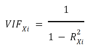
VIF values that exceed four are generally worthy of further investigation.
Options for dealing with multicollinearity include: dropping one of the collinear variables, or combining the two offending variables to form one composite measure. The latter option may not make sense in every situation.